Unified Algebra

A parsed query becomes a tree of operators. Each operator is a node from the unified algebra; the leaves are data sources and the root is the final result. This is the same algebra for every language; see Language Mapping for how each frontend gets here.

Operators come in two families:

• Tuple operators work on streams of named tuples, much like relational algebra (Selection, Projection, Join, ...).
• Item operators work on streams of opaque items.

A few operators (Limit, the set operators) work on either, depending on their input. The design draws on existing algebras for XQuery, graph paths, and nested relations.

The full catalog, with a plain-language description, signature, and formal semantics for each operator, lives in the Operator Reference. This page explains the concepts you need to read that catalog and the plans the engine produces.

Operator context

Some operators behave differently depending on the rows flowing through the operators around them. That surrounding state is the context, written $\Gamma \in \mathcal{T}$.

Think of $\Gamma$ as the variable scope an operator can see: the data that was available when it was created, plus the most recent tuples from its direct tuple-producing inputs. A correlated subquery, for instance, reads the outer row from its context.

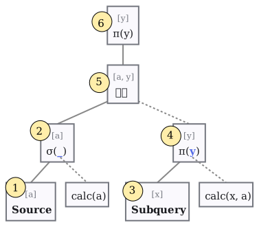
For example, see this simple plan. The operators receive the following context:

1. The bottom TupleSource gets no context.
2. The Selection (and the Calculation in its condition) gets the latest tuple from its source.
3. The subquery TupleSource gets the Selection's latest tuple.
4. The Projection and its Calculation receive the concatenation of the latest tuples produced by the Selection and the subquery TupleSource.
5. The ProjectionConcat receives the latest tuple from the Selection.
6. The top Projection receives the latest tuple from the ProjectionConcat.

In short: context flows down the tree, accumulating the rows each operator's ancestors have produced.

Instantiation: vertical vs. horizontal inputs

Operators differ in how often their inputs are (re)created, and this distinction drives both execution and how plans are drawn.

• Most inputs are created once and reused for the operator's whole life. These are vertical inputs ($\mathrm{vertical}(\mathrm{Op})$). Example: the source of a Selection. CartesianProduct likewise builds its left and right streams once.
• Some inputs are recreated repeatedly as the context changes, once per incoming row. These are horizontal inputs ($\mathrm{horizontal}(\mathrm{Op})$). Example: a correlated subquery inside a Selection condition.

Formally, a horizontal input is not a single stream but a stream indexed by context. We name this type with a constructor $\mathrm{inst}$: for any element type $X$,

$$\mathrm{inst}\,\mathrm{Stream}(X) \;:=\; \big(\mathcal{T} \rightarrow \mathrm{Stream}(X)\big).$$

A horizontal input of stream type $\mathrm{Stream}(X)$ therefore denotes an inhabitant of $\mathrm{inst}\,\mathrm{Stream}(X)$, a function $E : \mathcal{T} \rightarrow \mathrm{Stream}(X)$ supplied by the sub-plan, and instantiating it at a context $\Gamma$ is just application, $E(\Gamma)$. The same type has many inhabitants, one per sub-plan, so which stream you get for a given $\Gamma$ depends on which $E$ was supplied, not on $\Gamma$ alone.

You'll see the $\mathrm{inst}$ notation in operator signatures wherever an argument is re-instantiated per row.

Plan visualization

The DortDB GUI draws each plan as a tree. The root is the final query, the leaves are data sources, and nodes are colored by the language they came from. Tuple-operator nodes also show their schema (the grey brackets).

Edges tell you the instantiation kind at a glance:

• Solid edge: the child is created once, with its parent (a vertical input).
• Dashed edge: the child is recreated many times during the parent's life (a horizontal input).

For example, in SELECT x + 3 AS xplusthree FROM table1, the TupleSource table1 is created once (solid), while the Calculation for x + 3 is re-evaluated per row (dashed) and points at the attribute it produces, xplusthree.

Try it

The GUI is live at filipjezek.github.io/dortdb/showcase. Type a query and watch the plan build.

A tour of the operator families

For exact semantics, jump to the Operator Reference. This section gives you the lay of the land.

Item operators

Most item operators are calculation intermediaries; they never appear as standalone plan nodes. Instead they are the pieces a Calculation is built from.

Calculation is the workhorse: it represents any computed value, such as a projection expression or a selection condition. Its arguments can be attribute references or even whole plan operators, which is how subqueries get embedded into an expression. When a subquery is involved, the Calculation records whether it should yield at most one value or many.

The remaining item operators are data sources and MapToItem, which pulls one attribute out of each tuple to turn a tuple stream into an item stream.

Subqueries and the optimizer

A subquery starts life as a Calculation wrapping a Projection. The optimizer can lift that into an outer ProjectionConcat, and, if the subquery doesn't depend on the outer row, further into a plain left outer Join. Same result, progressively cheaper plans.

Tuple operators

These are the familiar relational operators (Selection, Projection, Join, CartesianProduct, OrderBy) plus a few that earn their own mention:

• ProjectionConcat (a.k.a. depend-join) re-runs a subquery for each source row and joins the results back. It's how correlated subqueries and LATERAL joins are expressed.

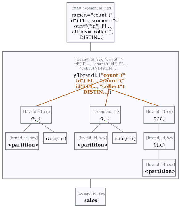
• GroupBy partitions rows by key and runs aggregates per partition. Each aggregate can carry its own filtering, ordering, or distinctness:

  SELECT
    count(id) FILTER (WHERE sex = 'M') AS men,
    count(id) FILTER (WHERE sex = 'F') AS women,
    collect(DISTINCT id ORDER BY id) AS all_ids
  FROM sales
  GROUP BY brand

• Recursion is a self-join repeated up to max times, executed breadth-first so the shortest results come out first. It powers variable-length graph paths and recursive CTEs.

XQuery-specific operators

ProjectionSize and TreeJoin ship with the XQuery package, not the core; they're the concrete proof that the algebra is extensible. TreeJoin implements path steps like a/b/c, exposing the XQuery focus ($fs:dot, $fs:position, $fs:last) for each step.

Universal operators

Union, Intersection, Difference, and Limit all work on tuples or items alike. NullSource emits a single empty row, which is what gives a constant query like SELECT 1 AS one something to project from.

Extensibility

The core algebra covers everything DortDB does today, but a new language might need more. When it does, adding an operator is just defining its behavior: you extend the relevant visitor classes inside your language package, and the core stays untouched. The XQuery operators above are built exactly this way.